Learning Objectives
In this section, you will:
- 3.4.1 – Identify exponential functions
- 3.4.2 – Evaluate exponential functions
- 3.4.3 – Graph exponential functions
India is the second most populous country in the world with a population of about [latex]\,1.25\,[/latex] billion people in 2013. The population is growing at a rate of about [latex]\,1.2%\,[/latex] each year[1] . If this rate continues, the population of India will exceed China’s population by the year [latex]\,2031.[/latex] When populations grow rapidly, we often say that the growth is “exponential,” meaning that something is growing very rapidly. To a mathematician, however, the term exponential growth has a very specific meaning. In this section, we will take a look at exponential functions, which model this kind of rapid growth.
3.4.1 – Identifying Exponential Functions
When exploring linear growth, we observed a constant rate of change—a constant number by which the output increased for each unit increase in input. For example, in the equation [latex]\,f\left(x\right)=3x+4,[/latex] the slope tells us the output increases by 3 each time the input increases by 1. The scenario in the India population example is different because we have a percent change per unit time (rather than a constant change) in the number of people.
Defining an Exponential Function
A study found that the percent of the population who are vegans in the United States doubled from 2009 to 2011. In 2011, 2.5% of the population was vegan, adhering to a diet that does not include any animal products—no meat, poultry, fish, dairy, or eggs. If this rate continues, vegans will make up 10% of the U.S. population in 2015, 40% in 2019, and 80% in 2021.
What exactly does it mean to grow exponentially? What does the word double have in common with percent increase? People toss these words around errantly. Are these words used correctly? The words certainly appear frequently in the media.
- Percent change refers to a change based on a percent of the original amount.
- Exponential growth refers to an increase based on a constant multiplicative rate of change over equal increments of time, that is, a percent increase of the original amount over time.
- Exponential decay refers to a decrease based on a constant multiplicative rate of change over equal increments of time, that is, a percent decrease of the original amount over time.
For us to gain a clear understanding of exponential growth, let us contrast exponential growth with linear growth. We will construct two functions. The first function is exponential. We will start with an input of 0, and increase each input by 1. We will double the corresponding consecutive outputs. The second function is linear. We will start with an input of 0, and increase each input by 1. We will add 2 to the corresponding consecutive outputs. See the table below.
| [latex]x[/latex] | [latex]f\left(x\right)={2}^{x}[/latex] | [latex]g\left(x\right)=2x[/latex] |
|---|---|---|
| 0 | 1 | 0 |
| 1 | 2 | 2 |
| 2 | 4 | 4 |
| 3 | 8 | 6 |
| 4 | 16 | 8 |
| 5 | 32 | 10 |
| 6 | 64 | 12 |
From this table we can infer that for these two functions, exponential growth dwarfs linear growth.
- Exponential growth refers to the original value from the range increases by the same percentage over equal increments found in the domain.
- Linear growth refers to the original value from the range increases by the same amount over equal increments found in the domain.
Apparently, the difference between “the same percentage” and “the same amount” is quite significant. For exponential growth, over equal increments, the constant multiplicative rate of change resulted in doubling the output whenever the input increased by one. For linear growth, the constant additive rate of change over equal increments resulted in adding 2 to the output whenever the input was increased by one.
The general form of the exponential function is [latex]\,f\left(x\right)=a{b}^{x},\,[/latex] where [latex]\,a\,[/latex] is any nonzero number, [latex]\,b\,[/latex] is a positive real number not equal to 1.
- If [latex]\,b>1,[/latex] the function grows at a rate proportional to its size.
- If [latex]\,0
Let’s look at the function [latex]\,f\left(x\right)={2}^{x}\,[/latex] from our example. We will create a table to determine the corresponding outputs over an interval in the domain from [latex]\,-3\,[/latex] to [latex]\,3.[/latex]
| [latex]x[/latex] | [latex]-3[/latex] | [latex]-2[/latex] | [latex]-1[/latex] | [latex]0[/latex] | [latex]1[/latex] | [latex]2[/latex] | [latex]3[/latex] |
| [latex]f\left(x\right)={2}^{x}[/latex] | [latex]{2}^{-3}=\frac{1}{8}[/latex] | [latex]{2}^{-2}=\frac{1}{4}[/latex] | [latex]{2}^{-1}=\frac{1}{2}[/latex] | [latex]{2}^{0}=1[/latex] | [latex]{2}^{1}=2[/latex] | [latex]{2}^{2}=4[/latex] | [latex]{2}^{3}=8[/latex] |
Let us examine the graph of [latex]\,f\,[/latex] by plotting the ordered pairs we observe on the table in Figure 1, and then make a few observations.
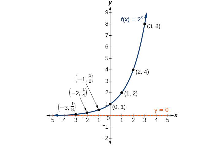
Let’s define the behavior of the graph of the exponential function [latex]\,f\left(x\right)={2}^{x}\,[/latex] and highlight some its key characteristics.
- the domain is [latex]\,\left(-\infty ,\infty \right),[/latex]
- the range is [latex]\,\left(0,\infty \right),[/latex]
- as [latex]\,x\to \infty ,f\left(x\right)\to \infty ,[/latex]
- as [latex]\,x\to -\infty ,f\left(x\right)\to 0,[/latex]
- [latex]\,f\left(x\right)\,[/latex] is always increasing,
- the graph of [latex]\,f\left(x\right)\,[/latex] will never touch the x-axis because base two raised to any exponent never has the result of zero.
- [latex]\,y=0\,[/latex] is the horizontal asymptote.
- the y-intercept is 1.
Exponential Function
For any real number [latex]\,x,[/latex] an exponential function is a function with the form
where
- [latex]\,a\,[/latex] is a non-zero real number called the initial value and
- [latex]\,b\,[/latex] is any positive real number such that [latex]\,b\ne 1.[/latex]
- The domain of [latex]\,f\,[/latex] is all real numbers.
- The range of [latex]\,f\,[/latex] is all positive real numbers if [latex]\,a>0.[/latex]
- The range of [latex]\,f\,[/latex] is all negative real numbers if [latex]\,a<0.[/latex]
- The y-intercept is [latex]\,\left(0,a\right),[/latex] and the horizontal asymptote is [latex]\,y=0.[/latex]
Example 1 – Identifying Exponential Functions
Which of the following equations are not exponential functions?
- [latex]f\left(x\right)={4}^{3\left(x-2\right)}[/latex]
- [latex]g\left(x\right)={x}^{3}[/latex]
- [latex]h\left(x\right)={\left(\frac{1}{3}\right)}^{x}[/latex]
- [latex]j\left(x\right)={\left(-2\right)}^{x}[/latex]
By definition, an exponential function has a constant as a base and an independent variable as an exponent. Thus, [latex]\,g\left(x\right)={x}^{3}\,[/latex] does not represent an exponential function because the base is an independent variable. In fact, [latex]\,g\left(x\right)={x}^{3}\,[/latex] is a power function.
Recall that the base b of an exponential function is always a positive constant, and [latex]\,b\ne 1.\,[/latex] Thus, [latex]\,j\left(x\right)={\left(-2\right)}^{x}\,[/latex] does not represent an exponential function because the base, [latex]\,-2,[/latex] is less than [latex]\,0.[/latex]
Try It
Which of the following equations represent exponential functions?
- [latex]f\left(x\right)=2{x}^{2}-3x+1[/latex]
- [latex]g\left(x\right)={0.875}^{x}[/latex]
- [latex]h\left(x\right)=1.75x+2[/latex]
- [latex]j\left(x\right)={1095.6}^{-2x}[/latex]
Show answer
[latex]g\left(x\right)={0.875}^{x}\,[/latex] and [latex]j\left(x\right)={1095.6}^{-2x}\,[/latex] represent exponential functions.
3.4.2 – Evaluating Exponential Functions
Recall that the base of an exponential function must be a positive real number other than [latex]\,1.[/latex] Why do we limit the base [latex]b\,[/latex] to positive values? To ensure that the outputs will be real numbers. Observe what happens if the base is not positive:
- Let [latex]\,b=-9\,[/latex] and [latex]\,x=\frac{1}{2}.\,[/latex] Then [latex]\,f\left(x\right)=f\left(\frac{1}{2}\right)={\left(-9\right)}^{\frac{1}{2}}=\sqrt{-9},[/latex] which is not a real number.
Why do we limit the base to positive values other than [latex]1?[/latex] Because base [latex]1\,[/latex] results in the constant function. Observe what happens if the base is [latex]1:[/latex]
- Let [latex]\,b=1.\,[/latex] Then [latex]\,f\left(x\right)={1}^{x}=1\,[/latex] for any value of [latex]\,x.[/latex]
To evaluate an exponential function with the form [latex]\,f\left(x\right)={b}^{x},[/latex] we simply substitute [latex]x\,[/latex] with the given value, and calculate the resulting power. For example:
Let [latex]\,f\left(x\right)={2}^{x}.\,[/latex] What is [latex]f\left(3\right)?[/latex]
[latex]$$\begin{array}{lll}f\left(x\right)\hfill & ={2}^{x}\hfill & \hfill \\ f\left(3\right)\hfill & ={2}^{3}\text{ }\hfill & \text{Substitute }x=3.\hfill \\ \hfill & =8\text{ }\hfill & \text{Evaluate the power}\text{.}\hfill \end{array}$$[/latex]
To evaluate an exponential function with a form other than the basic form, it is important to follow the order of operations. For example:
Let [latex]\,f\left(x\right)=30{\left(2\right)}^{x}.\,[/latex] What is [latex]\,f\left(3\right)?[/latex]
[latex]$$\begin{array}{lll}f\left(x\right)\hfill & =30{\left(2\right)}^{x}\hfill & \hfill \\ f\left(3\right)\hfill & =30{\left(2\right)}^{3}\hfill & \text{Substitute }x=3.\hfill \\ \hfill & =30\left(8\right)\text{ }\hfill & \text{Simplify the power first}\text{.}\hfill \\ \hfill & =240\hfill & \text{Multiply}\text{.}\hfill \end{array}$$[/latex]
Note that if the order of operations were not followed, the result would be incorrect:
[latex]$$f\left(3\right)=30{\left(2\right)}^{3}\ne {60}^{3}=216,000$$[/latex]
Example 2 – Evaluating Exponential Functions
Let [latex]\,f\left(x\right)=5{\left(3\right)}^{x+1}.\,[/latex] Evaluate [latex]\,f\left(2\right)\,[/latex] without using a calculator.
Follow the order of operations. Be sure to pay attention to the parentheses.
[latex]$$\begin{array}{lll}f\left(x\right)\hfill & =5{\left(3\right)}^{x+1}\hfill & \hfill \\ f\left(2\right)\hfill & =5{\left(3\right)}^{2+1}\hfill & \text{Substitute }x=2.\hfill \\ \hfill & =5{\left(3\right)}^{3}\hfill & \text{Add the exponents}.\hfill \\ \hfill & =5\left(27\right)\hfill & \text{Simplify the power}\text{.}\hfill \\ \hfill & =135\hfill & \text{Multiply}\text{.}\hfill \end{array}$$[/latex]
Try It
Let [latex]f\left(x\right)=8{\left(1.2\right)}^{x-5}.\,[/latex] Evaluate [latex]\,f\left(3\right)\,[/latex] using a calculator. Round to four decimal places.
Show answer
[latex]5.5556[/latex]
Defining Exponential Growth
Because the output of exponential functions increases very rapidly, the term “exponential growth” is often used in everyday language to describe anything that grows or increases rapidly. However, exponential growth can be defined more precisely in a mathematical sense. If the growth rate is proportional to the amount present, the function models exponential growth.
Exponential Growth
A function that models exponential growth grows by a rate proportional to the amount present. For any real number [latex]\,x\,[/latex] and any positive real numbers [latex]\,a \,[/latex] and [latex]\,b\,[/latex] such that [latex]\,b\ne 1,[/latex] an exponential growth function has the form
where
- [latex]a\,[/latex] is the initial or starting value of the function.
- [latex]b\,[/latex] is the growth factor or growth multiplier per unit [latex]\,x[/latex] .
In more general terms, we have an exponential function, in which a constant base is raised to a variable exponent. To differentiate between linear and exponential functions, let’s consider two companies, A and B. Company A has 100 stores and expands by opening 50 new stores a year, so its growth can be represented by the function [latex]\,A\left(x\right)=100+50x.\,[/latex] Company B has 100 stores and expands by increasing the number of stores by 50% each year, so its growth can be represented by the function [latex]\,B\left(x\right)=100{\left(1+0.5\right)}^{x}.[/latex]
A few years of growth for these companies are illustrated in the table below.
| Year, [latex]x[/latex] | Stores, Company A | Stores, Company B |
|---|---|---|
| [latex]0[/latex] | [latex]100+50\left(0\right)=100[/latex] | [latex]100{\left(1+0.5\right)}^{0}=100[/latex] |
| [latex]1[/latex] | [latex]100+50\left(1\right)=150[/latex] | [latex]100{\left(1+0.5\right)}^{1}=150[/latex] |
| [latex]2[/latex] | [latex]100+50\left(2\right)=200[/latex] | [latex]100{\left(1+0.5\right)}^{2}=225[/latex] |
| [latex]3[/latex] | [latex]100+50\left(3\right)=250[/latex] | [latex]100{\left(1+0.5\right)}^{3}=337.5[/latex] |
| [latex]x[/latex] | [latex]A\left(x\right)=100+50x[/latex] | [latex]B\left(x\right)=100{\left(1+0.5\right)}^{x}[/latex] |
The graphs comparing the number of stores for each company over a five-year period are shown in Figure 2. We can see that, with exponential growth, the number of stores increases much more rapidly than with linear growth.
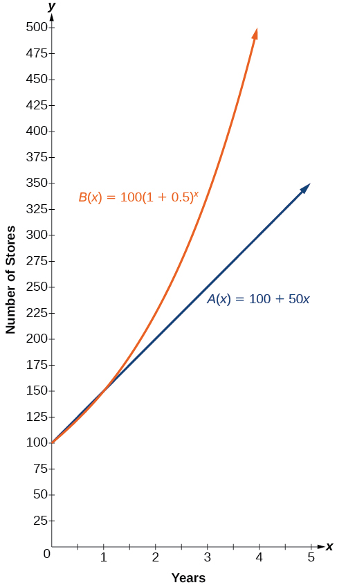
Notice that the domain for both functions is [latex]\,\left[0,\infty \right),[/latex] and the range for both functions is [latex]\,\left[100,\infty \right).\,[/latex] After year 1, Company B always has more stores than Company A.
Now we will turn our attention to the function representing the number of stores for Company B, [latex]\,B\left(x\right)=100{\left(1+0.5\right)}^{x}.\,[/latex] In this exponential function, 100 represents the initial number of stores, 0.50 represents the growth rate, and [latex]\,1+0.5=1.5\,[/latex] represents the growth factor. Generalizing further, we can write this function as [latex]\,B\left(x\right)=100{\left(1.5\right)}^{x},[/latex] where 100 is the initial value, [latex]\,1.5\,[/latex] is called the base, and [latex]\,x\,[/latex] is called the exponent.
Example 3 – Evaluating a Real-World Exponential Model
At the beginning of this section, we learned that the population of India was about [latex]\,1.25\,[/latex] billion in the year 2013, with an annual growth rate of about [latex]\,1.2%.\,[/latex] This situation is represented by the growth function [latex]\,P\left(t\right)=1.25{\left(1.012\right)}^{t},[/latex] where [latex]\,t\,[/latex] is the number of years since [latex]\,2013.\,[/latex] To the nearest thousandth, what will the population of India be in [latex]\,\text{2031?}[/latex]
To estimate the population in 2031, we evaluate the models for [latex]\,t=18,[/latex] because 2031 is [latex]\,18[/latex] years after 2013. Rounding to the nearest thousandth,
[latex]$$P\left(18\right)=1.25{\left(1.012\right)}^{18}\approx 1.549$$[/latex]
There will be about 1.549 billion people in India in the year 2031.
Try It
The population of China was about 1.39 billion in the year 2013, with an annual growth rate of about [latex]\,0.6%.\,[/latex] This situation is represented by the growth function [latex]\,P\left(t\right)=1.39{\left(1.006\right)}^{t},[/latex] where [latex]\,t\,[/latex] is the number of years since [latex]\,2013.[/latex] To the nearest thousandth, what will the population of China be for the year 2031? How does this compare to the population prediction we made for India in Example 3?
Show answer
About [latex]\,1.548\,[/latex] billion people; by the year 2031, India’s population will exceed China’s by about 0.001 billion, or 1 million people.
3.4.3 – Graphing Exponential Functions
Before we begin graphing, it is helpful to review the behavior of exponential growth. Recall the table of values for a function of the form [latex]\,f\left(x\right)={b}^{x}\,[/latex] whose base is greater than one. We’ll use the function [latex]\,f\left(x\right)={2}^{x}.\,[/latex] Observe how the output values in the table below change as the input increases by [latex]\,1.[/latex]
| [latex]x[/latex] | [latex]-3[/latex] | [latex]-2[/latex] | [latex]-1[/latex] | [latex]0[/latex] | [latex]1[/latex] | [latex]2[/latex] | [latex]3[/latex] |
| [latex]f\left(x\right)={2}^{x}[/latex] | [latex]\frac{1}{8}[/latex] | [latex]\frac{1}{4}[/latex] | [latex]\frac{1}{2}[/latex] | [latex]1[/latex] | [latex]2[/latex] | [latex]4[/latex] | [latex]8[/latex] |
Each output value is the product of the previous output and the base, [latex]\,2.\,[/latex] We call the base [latex]\,2\,[/latex] the constant ratio. In fact, for any exponential function with the form [latex]\,f\left(x\right)=a{b}^{x},[/latex] [latex]\,b\,[/latex] is the constant ratio of the function. This means that as the input increases by 1, the output value will be the product of the base and the previous output, regardless of the value of [latex]\,a.[/latex]
Notice from the table that
- the output values are positive for all values of [latex]x;[/latex]
- as [latex]\,x\,[/latex] increases, the output values increase without bound; and
- as [latex]\,x\,[/latex] decreases, the output values grow smaller, approaching zero.
Figure 7 shows the exponential growth function [latex]\,f\left(x\right)={2}^{x}.[/latex]
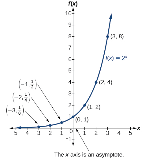
The domain of [latex]\,f\left(x\right)={2}^{x}\,[/latex] is all real numbers, the range is [latex]\,\left(0,\infty \right),[/latex] and the horizontal asymptote is [latex]\,y=0.[/latex]
To get a sense of the behavior of exponential decay, we can create a table of values for a function of the form [latex]\,f\left(x\right)={b}^{x}\,[/latex] whose base is between zero and one. We’ll use the function [latex]\,g\left(x\right)={\left(\frac{1}{2}\right)}^{x}.\,[/latex] Observe how the output values in the table below change as the input increases by [latex]\,1.[/latex]
| [latex]x[/latex] | [latex]-3[/latex] | [latex]-2[/latex] | [latex]-1[/latex] | [latex]0[/latex] | [latex]1[/latex] | [latex]2[/latex] | [latex]3[/latex] |
| [latex]g(x)=\left(\frac{1}{2}\right)^{x}[/latex] | [latex]8[/latex] | [latex]4[/latex] | [latex]2[/latex] | [latex]1[/latex] | [latex]\frac{1}{2}[/latex] | [latex]\frac{1}{4}[/latex] | [latex]\frac{1}{8}[/latex] |
Again, because the input is increasing by 1, each output value is the product of the previous output and the base, or constant ratio [latex]\,\frac{1}{2}.[/latex]
Notice from the table that
- the output values are positive for all values of [latex]\,x;[/latex]
- as [latex]\,x\,[/latex] increases, the output values grow smaller, approaching zero; and
- as [latex]\,x\,[/latex] decreases, the output values grow without bound.
Figure 8 shows the exponential decay function, [latex]\,g\left(x\right)={\left(\frac{1}{2}\right)}^{x}.[/latex]
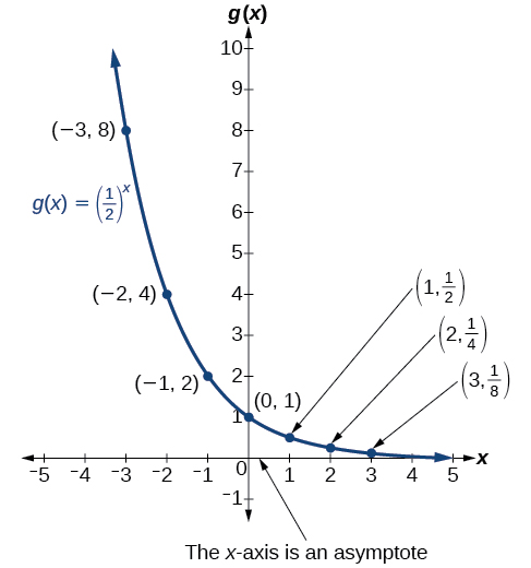
The domain of [latex]\,g\left(x\right)={\left(\frac{1}{2}\right)}^{x}\,[/latex] is all real numbers, the range is [latex]\,\left(0,\infty \right),[/latex] and the horizontal asymptote is [latex]\,y=0.[/latex]
Characteristics of the Graph of the Parent Function f(x) = bx
An exponential function with the form [latex]\,f\left(x\right)={b}^{x},[/latex] [latex]\,b>0,[/latex] [latex]\,b\ne 1,[/latex] has these characteristics:
- one-to-one function
- horizontal asymptote: [latex]\,y=0[/latex]
- domain: [latex]\,\left(–\infty , \infty \right)[/latex]
- range: [latex]\,\left(0,\infty \right)[/latex]
- x-intercept: none
- y-intercept: [latex]\,\left(0,1\right)\,[/latex]
- increasing if [latex]\,b>1[/latex]
- decreasing if [latex]\,b<1[/latex]
Figure 9 compares the graphs of exponential growth and decay functions.
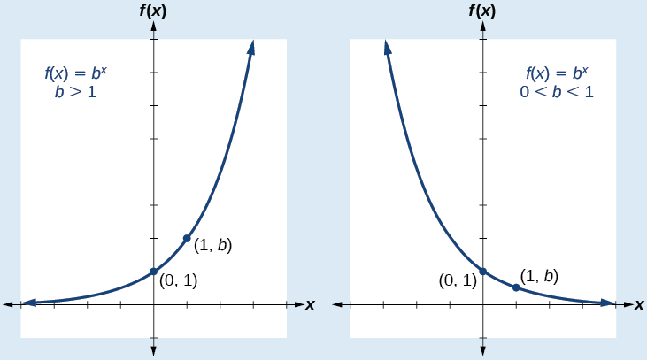
How To
Given an exponential function of the form [latex]\,f\left(x\right)={b}^{x},[/latex] graph the function.
- Create a table of points.
- Plot at least [latex]\,3\,[/latex] point from the table, including the y-intercept [latex]\,\left(0,1\right).[/latex]
- Draw a smooth curve through the points.
- State the domain, [latex]\,\left(-\infty ,\infty \right),[/latex] the range, [latex]\,\left(0,\infty \right),[/latex] and the horizontal asymptote, [latex]\,y=0.[/latex]
Example 4 – Sketching the Graph of an Exponential Function of the Form f(x) = bx
Sketch a graph of [latex]\,f\left(x\right)={0.25}^{x}.\,[/latex] State the domain, range, and asymptote.
Before graphing, identify the behavior and create a table of points for the graph.
- Since [latex]\,b=0.25\,[/latex] is between zero and one, we know the function is decreasing. The left tail of the graph will increase without bound, and the right tail will approach the asymptote [latex]\,y=0.[/latex]
- Create a table of points.
[latex]x[/latex] [latex]-3[/latex] [latex]-2[/latex] [latex]-1[/latex] [latex]0[/latex] [latex]1[/latex] [latex]2[/latex] [latex]3[/latex] [latex]f\left(x\right)={0.25}^{x}[/latex] [latex]64[/latex] [latex]16[/latex] [latex]4[/latex] [latex]1[/latex] [latex]0.25[/latex] [latex]0.0625[/latex] [latex]0.015625[/latex] - Plot the y-intercept, [latex]\,\left(0,1\right),[/latex] along with two other points. We can use [latex]\,\left(-1,4\right)\,[/latex] and [latex]\,\left(1,0.25\right).[/latex]
Draw a smooth curve connecting the points as in Figure 10.

The domain is [latex]\,\left(-\infty ,\infty \right);\,[/latex] the range is [latex]\,\left(0,\infty \right);\,[/latex] the horizontal asymptote is [latex]\,y=0.[/latex]
Try It
Sketch the graph of [latex]\,f\left(x\right)={4}^{x}.\,[/latex] State the domain, range, and asymptote.
Show answer
The domain is [latex]\,\left(-\infty ,\infty \right);\,[/latex] the range is [latex]\,\left(0,\infty \right);\,[/latex] the horizontal asymptote is [latex]\,y=0.[/latex]

Access these online resources for additional instruction and practice with exponential functions.
Key Equations
| definition of the exponential function | [latex]f\left(x\right)={b}^{x}\text{, where }b>0, b\ne 1[/latex] |
| definition of exponential growth | [latex]f\left(x\right)=a{b}^{x},\text{ where }a>0,b>0,b\ne 1[/latex] |
Key Concepts
- An exponential function is defined as a function with a positive constant other than [latex]\,1\,[/latex] raised to a variable exponent. See Example 1.
- A function is evaluated by solving at a specific value. See Example 2 and Example 3.
- The graph of the function [latex]\,f\left(x\right)={b}^{x}\,[/latex] has a y-intercept at [latex]\,\left(0, 1\right),[/latex] domain [latex]\,\left(-\infty , \infty \right),[/latex] range [latex]\,\left(0, \infty \right),[/latex] and horizontal asymptote [latex]\,y=0.\,[/latex] See Example 4.
- If [latex]\,b>1,[/latex] the function is increasing. The left tail of the graph will approach the asymptote [latex]\,y=0,[/latex] and the right tail will increase without bound.
- If [latex]\,0
Glossary
- exponential growth
- a model that grows by a rate proportional to the amount present
- http://www.worldometers.info/world-population/. Accessed February 24, 2014. ↵
